line AB is higher utility than the indifference curve.
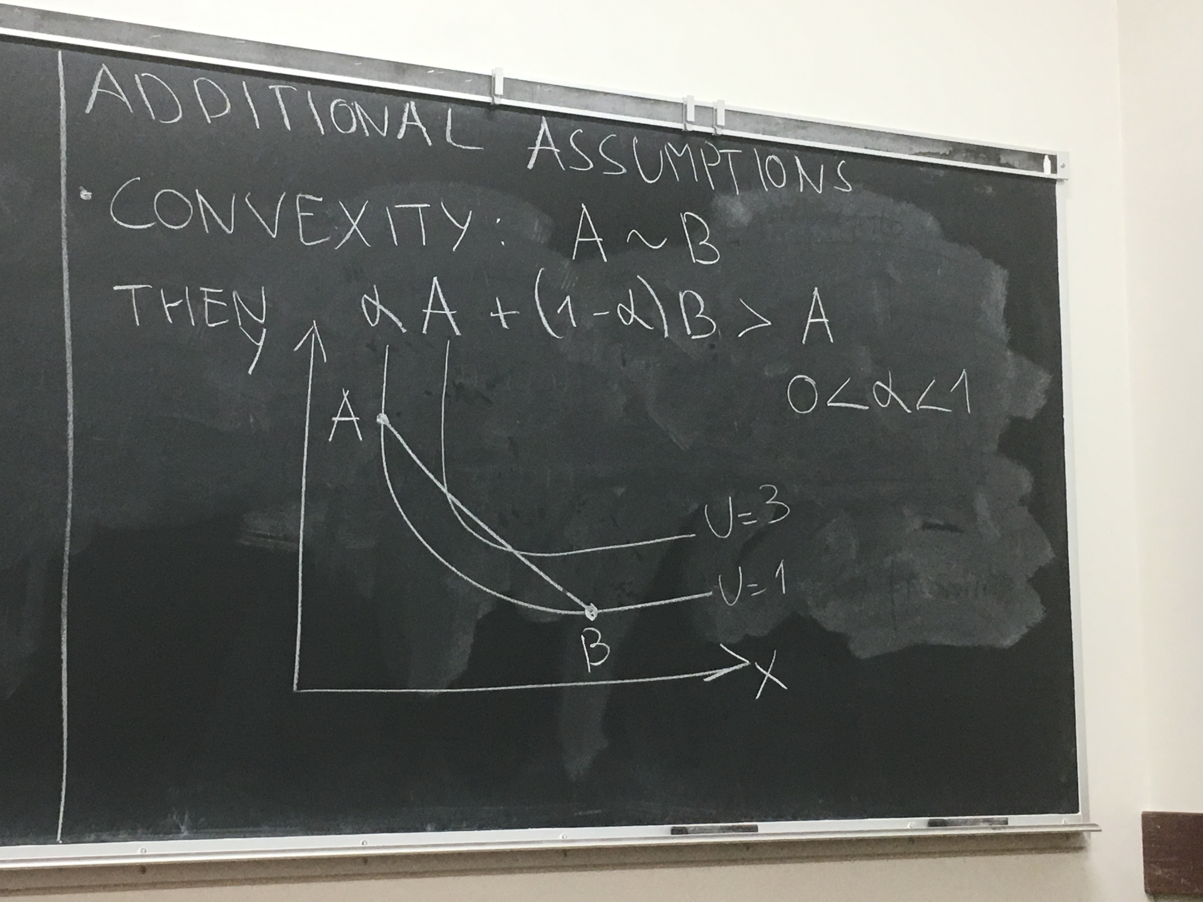
how people make decisions.
Example:
| A: 0.3 carat Dimond Ring | B: 3 carat Dimond Ring |
|---|---|
| Let: | |
| multiple by 2 | |
| multiple by power of 2 | |
| log |
→ U(B) > U(A)$ for most people. (the desire of B)
→ Imply a increasing function.
Indifference Curve shows a set of consumption bundles among which the individual is indifferent.
Marginal rate of substitution, MRS, the negative of the slope of the indifference curve at any point. .
Example: All , such that ;
Total differential ;
no intersection.

, and given: ,
→
therefore,
therefore:
Tangent condition
(holds to many goods)
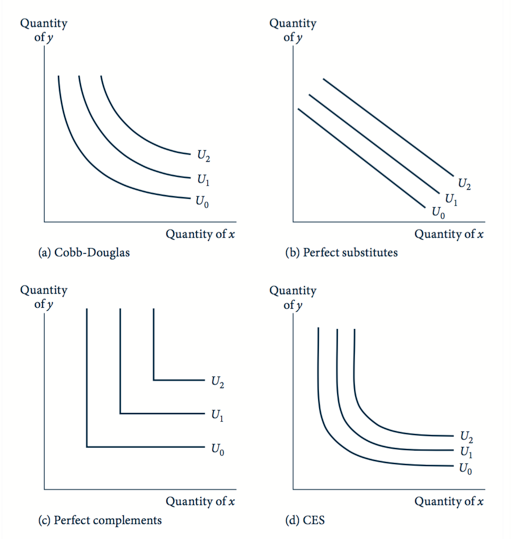
Perfect substitutes:
no larganian can be appliedPerfect Complements:
.
The Angle gives the right combination, any other point does not change the utility.
Constant Elasticity of substitution:
previous three are special cases of CES.
.
Homothetic Preferences: MRS
Non Homothetic Preferences: MRS = y
= K, Constant
Set two goods, are the price of two goods, income , then we have
when , vertical intersection.
when , horizontal intersection.
Connect the points then we get the bundles we can choose.
, slope is negative.
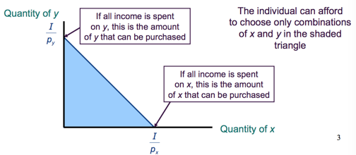
Example:
= drink, duck, = 20/lB
then we have = 100/20 = -5, meaning that for one more drink we receive, we need to give up one pound of duck.

Utility is maximized at B.
The budget constrain and the tangent line have same slope.
slope of budget constraint
slope of indifference curve
then we have
Example:
Need to find the Max of ,
Then we can set up
Take Partial derivatives equals Zero, so that
→ ;
MRS is diminishing: Convax → Always have a maximum;
MRS is not diminishing: Check second order derivatives;
When increase x, MRS is flatter, how to check:
Maximize utility by choosing to consume only one of the goods, where the indifference curve is not tangent to the budget constraint.
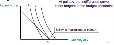
in this class, when we get the max from first order derivative, then there is no need to check second order, except 2 following situations:
Let = Food with = other goods with , the utility function is
→ then we can set up:
→ set first order derivative equals zero:
→ , plug in and solve for and
→ , similar:
$g_1, g_2$ are Marshallian Demand Funciton
Then we check second order derivatives:
indifference curve is flatter than the budget constraint:
;
indifference curve is steeper than the budget constraint:
;
Given
(How to find out the indifference curve is flatter or steeper?)
slope indifference curve:
Given , we need to find the max of U, min
→ set ,
and on the budget constraint.
→ solve:
and .
How the welfare/utility change when the price and income vary. Need to find the optimal consumption, replace in Utility and we get indire utility function , denoted as .
Enable us to determine the effect of government policies on the welfare/happiness of an individual.
Example:
, and given
so we can calculate
→
Example:
Policy: Progresa pays 200$ a year to eligible families that pay money for education.(Mexico reduces poverty).
Known: Average income: 13200 pesos = 1320$ (1 peso = 0.1$), Hourly wage = 0.1$, Price of consumption: 0.1$, Cobb Douglas
Utility Function,
Before government involves:
With the 200$ cash from government:
Price subsidy → 200 per family
, → the price of goods
now is changed to .
∴ , →
→
Compare the above results:
Example:
let be two goods and be their price, the Expenditure , with slope , and therefore
then the problem becomes to solove the minimum
for: min ,
→
Continue to buy same set of goods as changes, his expenditure function would be .
Actual expenditure is less expensive than by reallocating consumption to goods.
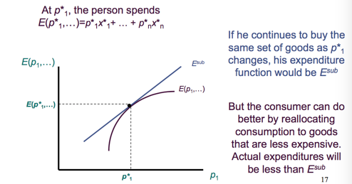
min pc+wl →
→
$U(c,l)=c^{0.5}l^{0.5}
→
Utility Maximization
Expenditure Minimization
Example:
→
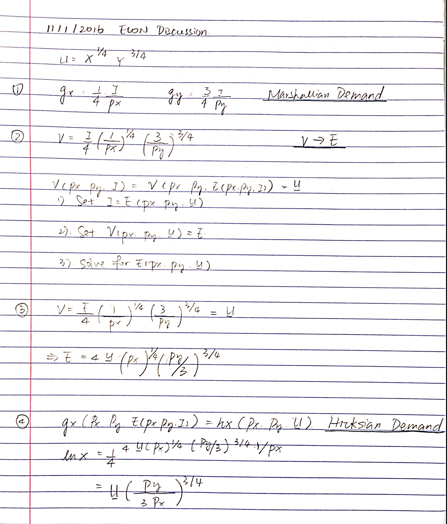
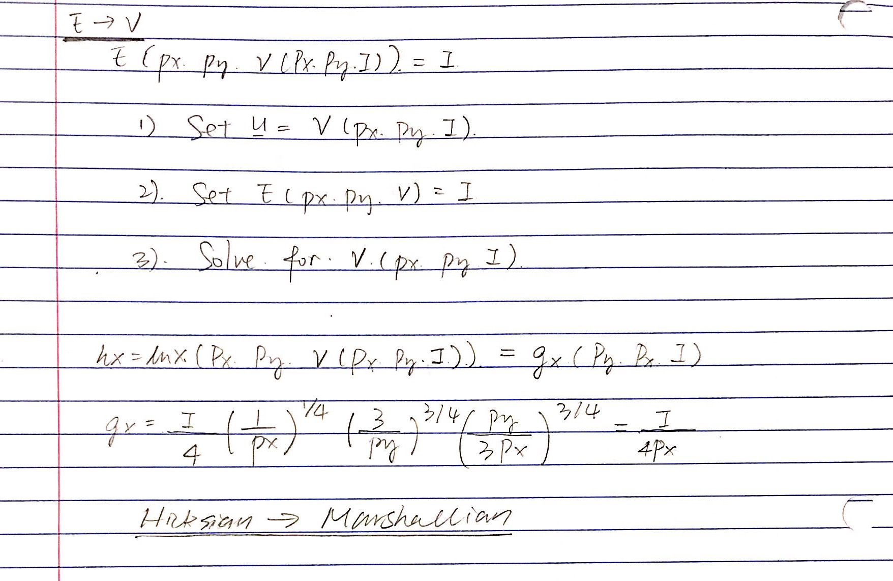
Example: from last lecture.
→ derive → derive
Then we get , therefore
